Lab 12: Inverted Pendulum
11 minutes read •
Overview
I drew inspiration from two prior writeups — Aravind Ramaswami's wheelie report (Kalman + pole-placement) and Stephan Wagner's Lab 12 report (hand-tuned PD, no observer). With Dyllan Hofflich and Tina Cheng, our final solution lands closer to Stephan's.
The inverted pendulum is a very famous unstable nonlinear system — a small disturbance from vertical grows exponentially unless the controller can inject a corrective force faster than the car falls. On our hardware the fall-time constant is about 70 ms, which sets a hard lower bound on the control loop rate. The lab broke into three pieces: model the car as a pendulum on a cart, build a real-time balance controller at $\theta = 0$, and add a launch state machine to flip the car up from horizontal.
System Modeling
Pendulum-on-cart geometry
A wheel of mass $M$ translates along $x$, with a rigid rod of mass $m$ and moment of inertia $I$ attached to its axle. The rod's COM is a distance $\ell$ above the wheel center. State vector:
$$ \mathbf{x} = \begin{bmatrix} x \ \dot x \ \theta \ \dot\theta \end{bmatrix}. $$
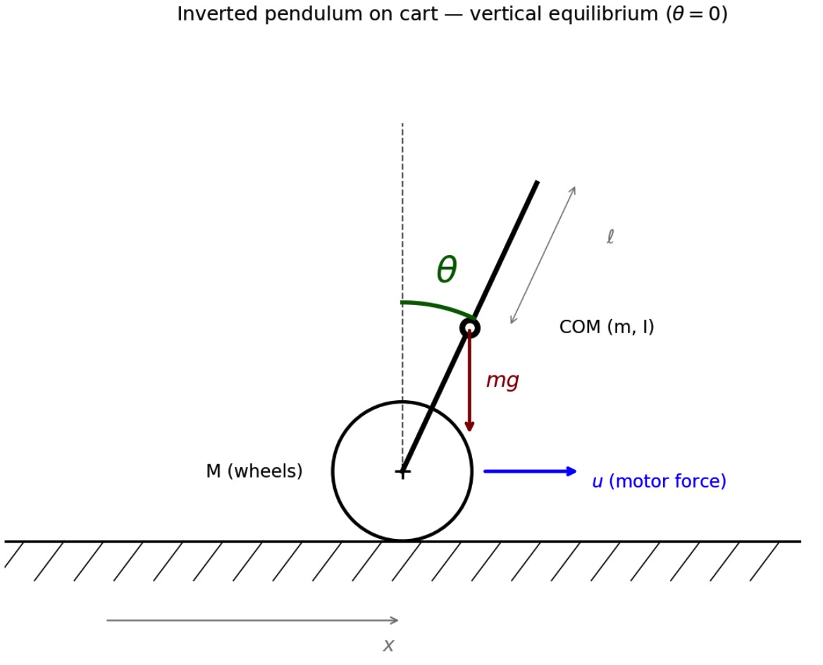
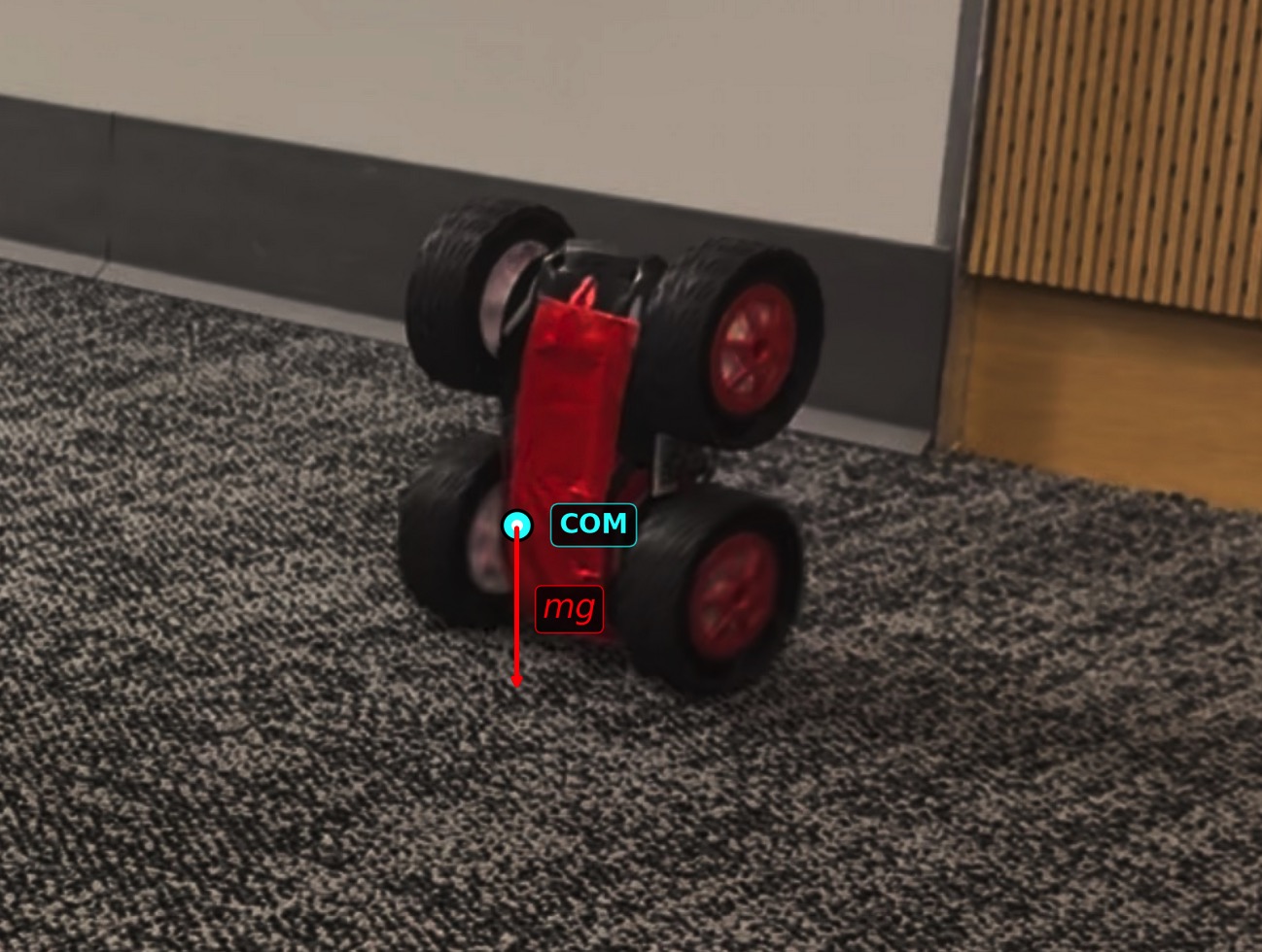
Lagrangian and equations of motion
With $T_w = \tfrac{1}{2}M\dot x^2$, $T_p = \tfrac{1}{2}m,[(\dot x + \ell\dot\theta\cos\theta)^2 + (\ell\dot\theta\sin\theta)^2] + \tfrac{1}{2}I\dot\theta^2$, and $V = mg\ell\cos\theta$, the Lagrangian $\mathcal{L} = T_w + T_p - V$ gives:
$$ (M + m),\ddot x + m\ell,\ddot\theta\cos\theta - m\ell,\dot\theta^2\sin\theta = u $$ $$ (I + m\ell^2),\ddot\theta + m\ell,\ddot x\cos\theta - mg\ell\sin\theta = 0 $$
Linearization about vertical
Substituting $\sin\theta \approx \theta$, $\cos\theta \approx 1$, $\dot\theta^2 \approx 0$ linearizes the coupled equations around the upright equilibrium. Since the car has no wheel encoder and I can't ready the cart's absolute position, I drop the $x$ row entirely — penalizing $x$ in $Q$ wouldn't actually make the controller know where the cart is. The reduced 2-state model in $[\theta,\ \dot\theta]$ becomes:
$$ \dot{\mathbf{x}} = A\mathbf{x} + B u, \quad A = \begin{bmatrix} 0 & 1 \ \alpha_1 & 0 \end{bmatrix}, \quad B = \begin{bmatrix} 0 \ \alpha_2 \end{bmatrix} $$
with $\alpha_1, \alpha_2$ aggregating $g$, $\ell$, $m$, $M$, $I$. The positive entry $\alpha_1$ on the off-diagonal is what makes the upright equilibrium unstable — its square root is the divergent eigenvalue of $A$, the reciprocal of the fall-time constant. I initialize $\alpha_1 \approx 6.21$, $\alpha_2 \approx 60$ from Aravind's report as a starting point.
I will retune the constants by hands later.
Controller Design
LQR for principled gain selection
LQR produces gains that optimally trade off state error against control effort. The cost $J = \int_0^\infty \mathbf{x}^\top Q,\mathbf{x} + R u^2, dt$ gives optimal feedback $K = R^{-1} B^\top P$, where $P$ solves the continuous-time algebraic Riccati equation:
$$ A^\top P + P A - P B R^{-1} B^\top P + Q = 0. $$
I weighted $Q$ heavily on $\theta$ (100) and lightly on $\dot\theta$ (1), with $R = 1$ — penalize pose error, tolerate motion, don't over-penalize the motor:
import numpy as np
from scipy.linalg import solve_continuous_are

A = np.array([[0, 1], [6.21, 0]])
B = np.array([[0], [60.0]])
Q = np.diag([100.0, 1.0])
R = np.array([[1.0]])

P = solve_continuous_are(A, B, Q, R)
K = np.linalg.inv(R) @ B.T @ P
print("LQR gains [Kp, Kd]:", K.ravel())
Result: $K_p \approx 0.04$, $K_d \approx 0.005$
Why PD with hand-tuned gains in the end
The LQR output assumes the control input is in Newtons, but my firmware issues signed PWM (−255 to +255). Converting between them requires a force-to-PWM constant $k_f$ that I never measured, which left my LQR gains dimensionally inconsistent with the motor command. I converged on PD gains by hand instead, using the LQR ratio of $K_p:K_d$ as a starting point:
| Parameter | Value | Why |
|---|---|---|
| $K_p$ | 15.0 | 5° error → 75 PWM, above motor deadband |
| $K_d$ | 1.0 | Rate damping to avoid oscillation |
| max pwm | 255 | Full authority for large disturbances |
| target pitch | +90° | Wheelie orientation in my IMU mounting |
The reference's $K_p = 4$, $K_d = 0.2$ were sub-deadband: 5° → 20 PWM didn't move the wheels at all, then larger errors slammed past — a limit-cycle recipe. Tripling $K_p$ moved every meaningful correction above the motor's static-friction threshold.
Control law in firmware
if (stunt_state == IPEND_HOLD) {
    float pitch_rate_dps = +latest_gx;
    float deviation      = latest_pitch_comp - ipend_cfg.target_pitch_deg;
    float u              = ipend_cfg.Kp * deviation
                         + ipend_cfg.Kd * pitch_rate_dps;
    int   pwm            = (int)constrain(u, -ipend_cfg.max_pwm,
                                              +ipend_cfg.max_pwm);
    setLeftMotor(pwm);
    setRightMotor(pwm);
}
Both wheels get the same signed PWM — no differential needed.
IMU State Estimation
I tried Aravind's Kalman observer first, but the estimate drifted unpredictably during fast maneuvers — translational acceleration from the cart kept contaminating the accelerometer pitch, the filter couldn't distinguish it from a true tilt, and the controller would saturate on phantom angles. After a couple of sessions tuning $\Sigma_u$ and $\Sigma_z$ to no avail, I went back to the complementary filter I already used in earlier labs:
pitch_lpf_state = ALPHA_LPF * pitch_acc + (1 - ALPHA_LPF) * pitch_lpf_state;
pitch_comp_state = (1 - ALPHA_COMP) * (pitch_comp_state + pitch_rate * dt)
                 + ALPHA_COMP * pitch_lpf_state;
The intuition is that the gyro is accurate on short timescales but drifts when integrated; the accelerometer is noisy on short timescales but absolute on long ones. With ALPHA_LPF = 0.10 and ALPHA_COMP = 0.05, the filter trusts the gyro between frames and gently pulls toward the accel pitch over hundreds of milliseconds. At 50 Hz this is essentially as good as Kalman, with zero hyperparameters to retune per stunt.
Axis-swap calibration
My IMU was mounted rotated 90° about the car z-axis, so car pitch showed up on IMU-y instead of IMU-x. I verified this by walking the car through five orientations and noting which accel channel saturated to ±1 g in each. Fixed by swapping which axes feed pitch and roll:
latest_pitch_acc = atan2(latest_ay, latest_az) * 180.0f / M_PI;
latest_roll_acc  = atan2(latest_ax, latest_az) * 180.0f / M_PI;
float pitch_rate = +latest_gx;
Switching Cars + Tuning
After days of fighting motor deadband and surface friction on my own car, I switch to path planning on the last day to have a complete deliverable. Coming back to the pendulum with Dyllan and Tina, we ran my PD code on Dyllan's car and it balanced for a couple of seconds, my controller was actually decent for Ananya's car. We then committed to Dyllan's full LQR formulation and tuned it together; the results below come from his car. Ultimately, it came down to whose code seemed to have a better balance results because what it is left was just tuning, and it seems like his code just provided a better starting point
Wheelie Launch State Machine - Attempt
The launch sequence: drive forward to build linear momentum, brake hard to plant the front wheels, then reverse the motors. The wheels yank the contact point backward while the car's inertia keeps it moving forward, and the mismatch generates a forward-pitching torque about the front axle that lifts the rear into a wheelie. Once $|\theta| > 30°$, the FSM hands off to the balance controller. The FSM has one interesting state (BALANCE); everything else is event-driven timing, with timeouts dropping back to IDLE if the launch fails.
struct WheelieConfig {
    int   forward_pwm        = 250;
    int   forward_ms         = 250;
    int   brake_ms           = 100;
    int   reverse_pwm        = 250;
    int   reverse_ms         = 270;
    int   wait_max_ms        = 600;
    float balance_trigger_deg = 30.0f;
    float target_pitch_deg    = +90.0f;
    float Kp = 15.0f;
    float Kd = 1.0f;
    int   max_balance_pwm = 255;
};
Results
My best controller
Here's what my best inverted pendulum on Ananya's car. This is purely the code I developed on my own.
First attempt
We found that the performance of the controller with the initial gain matrix was pretty bad, with the robot oscillating a lot and not being able to balance for more than a second if at all.
After tuning
Instead of trying to tune the Q and R matrices to get a better gain matrix, we decided to just manually tune the gain matrix by hand.
PID solution
After struggling to get the LQR controller to work well, we attempted to implement a PID controller on a linearized system. It is a simple PID controller using the angle error from the DMP readings, we thought we had more experience tuning it from previous labs, but it just performed worse.
Launch attempts
Two attempts at the full launch-to-balance logic. The launch FSM reaches the trigger threshold, but the dynamic was super noisy, and our balance controller cannot handle it very well.
Surface comparison: wood vs. carpet
Surface friction matters more than I expected. On wood the wheels slip during accelerations, so the controller cannot change fast enough, and the car tends to be less stable. On carpet the wheels bite and the controller's output actually moves the cart, which is what makes balance sustainable.
Best result on wood:
Best results on carpet:
Final results — with weight on top
The breakthrough was taping weights to the top of the chassis(with some further tuning of course). The higher $I_{b,\text{com}}$ lengthens the fall-time constant, which gives the controller more headroom to react to each disturbance. The pole has a much better stability. See the final clips at the bottom of Dyllan's Lab 12 report for the best runs of the tuned LQR with weight added.
Bonus Videos & Bloopers
Some of the more failures and side experiments from the tuning sessions.
Tangent: Path Planning
Overview of path planning. I worked on this for about six hours before joining Dyllan and Tina on the Inverted Pendulum. The task is to navigate 9 waypoints across the mapped arena, from $(-4, -3)$ to $(0, 0)$ in grid cells. I went with turn-go-turn between adjacent waypoints (no global planning — the waypoints are hand-designed and have no walls between consecutive points) and a Bayes-filter update at every waypoint, reusing the Lab 11 pattern: uniform-prior reset before each 360° scan, no prediction step (the provided $O(N^6)$ implementation is too slow for online use). Onboard PID handles both the in-place turn and the ToF-based straight leg; offboard Python plans the segments and awaits DONE notifications from the firmware so the Bayes-filter compute doesn't compete with the 50 Hz control loop. A single waypoint takes 8–12 seconds end-to-end, dominated by the 18 turn-and-settle cycles of the localization scan. My best run hits the first 4–5 waypoints before cumulative heading drift (±5° per turn) points the car at a wall.
async def step_once(self):
    # 1. Current pose = argmax of latest belief
    cell = np.unravel_index(np.argmax(self.loc.bel), self.loc.bel.shape)
    current_pose = self.loc.mapper.from_map(*cell)

    # 2. Turn-go-turn to next waypoint
    rot1, trans = self._plan_segment(current_pose, self.target_waypoint)
    await self.robot.turn_to_heading(current_pose[2] + rot1)
    await self.robot.drive_distance(trans)

    # 3. Re-localize: 360° scan + Bayes update
    await self.loc.get_observation_data()
    self.loc.update_step()
Collaboration
Thanks to Dyllan Hofflich for letting me run my PD code on Ananya Jajodia's car and working together with Dyllan Hofflich and Tina Cheng on the LQR derivation and tuning sessions. Thanks to Claude for helping debugging my inverted pendulum code and tuning process. Thanks to Professor Helbling and the entire teaching team of Fast Robots for a great semester. This is one of the best classes I have taken in college.